
Classification metrics quantitatively measure an Artificial Intelligence (AI) model's performance, highlighting its strengths and weaknesses, and help assess how well a deep learning model categorizes data into different classes.
Various classification metrics are used in deep learning, each serving a specific purpose. The most commonly used metrics include accuracy, precision, recall, F1 score, ROC-AUC, and Matthews correlation coefficient. This article focuses on accuracy, precision, and recall due to their widespread use and significance.
We will discuss their definitions, calculations, advantages, and disadvantages and compare them to help you make informed decisions when developing and evaluating deep learning models. Before we discuss these classifications, let's first understand the confusion matrix.
Confusion Matrix
A confusion matrix, also known as an error matrix, is a table that summarizes the performance of a classification model. It provides a detailed breakdown of the model's predictions versus the actual (true) labels. It's a square matrix where the rows represent the exact classes, and the columns represent the predicted classes.
Structure of a Confusion Matrix:
| Predicted Positive (PP) | Predicted Negative (PN) | |
|---|---|---|
| Actual Positive | True Positive (TP) | False Negative (FN) |
| Actual Negative | False Positive (FP) | True Negative (TN) |
Elements of a Confusion Matrix:
- True Positive (TP): The number of instances where the model correctly predicted a positive class.
- True Negative (TN): The number of instances where the model correctly predicted a negative class.
- False Positive (FP): The number of instances where the model incorrectly predicted a positive class (Type I error).
- False Negative (FN): The number of instances where the model incorrectly predicted a negative class (Type II error).
Here is an example of how it looks:

Interpreting a Confusion Matrix:
- The main diagonal (TP and TN) represents correct predictions.
- The off-diagonal elements (FP and FN) represent incorrect predictions.
- The row sums give the total number of actual instances in each class.
- The column sums provide the total number of predicted instances in each class.
For example, imagine you have a spam filter, and you test it on 1,000 emails, and the model does the following:
- Correctly identified 80 as spam
- Correctly identified 890 as not spam
- Incorrectly identified 10 as spam
- Incorrectly identified 20 as not spam
Here's how the confusion matrix would look:

Metrics Derived from a Confusion Matrix:
- Accuracy: The overall proportion of correct predictions.
- Precision: The proportion of positive predictions that were actually correct.
- Recall (Sensitivity): The proportion of actual positives that were correctly identified.
- Specificity: The proportion of actual negatives that were correctly identified.
- F1 Score: The harmonic mean of precision and recall, providing a balanced measure of performance.
Now that you understand confusion matrix, let us discuss accuracy classification.
Accuracy
Accuracy is one of the most straightforward and commonly used metrics in classification problems. It is defined as the ratio of correctly predicted instances to the total instances in the dataset. Mathematically, it can be represented as:

Accuracy is measured on a scale of 0 to 1 or as a percentage. The higher the accuracy, the better. It is possible to achieve a perfect accuracy of 1.0 when every prediction the model makes is correct. The accuracy metric helps get a quick sense of overall model performance, especially when the classes are balanced.
Here is how accuracy works in a binary classification problem where a model predicts whether a social media comment is positive or negative:
If a model is tasked to predict if social media comments on a post are positive or negative from 100 comments, when accuracy classification is used, the model will use a confusion matrix to determine what is positive or negative.
If the model correctly identifies 9 negative comments and positive comments out of a total of 100 comments, the accuracy would be:


However, it's important to note that accuracy might not always provide a complete picture of model performance, especially in cases where the class distribution is skewed. For instance, class imbalance is common in fraud detection, with fraudulent transactions making up a small fraction of all transactions. A high accuracy rate might not indicate good performance in identifying fraudulent activities. Here is an example:
If 97 out of 100 transactions are legitimate, a model predicting every transaction as legitimate will achieve 97% accuracy and fail to detect fraud.

This is because the accuracy metric calculates the percentage of correct predictions out of all predictions made. Since 97 out of 100 transactions are correctly identified as legitimate, the accuracy is 97%.
Pros and cons of accuracy classification
Pros:
- Simplicity: Accuracy is easy to understand and calculate, making it accessible to both technical and non-technical stakeholders.
- Intuitive: It provides a general sense of the model's performance, which can be useful for initial model assessment.
Cons:
- Lack of Detail: Accuracy does not provide information on the types of errors the model is making. It treats false positives and false negatives equally, which may not be appropriate for all applications.
Now that we know accuracy treats false positives and false negatives equally, let’s examine how precision resolves this.
Precision
Precision, also known as the positive predictive value (PPV), is a classification metric that focuses on the accuracy of positive predictions. It measures the proportion of instances the model predicted as positive that were true positives. Mathematically, it's defined as:

Precision ranges from 0 to 1, with higher values indicating better performance. A perfect precision of 1.0 means the model correctly identifies every positive instance without any false positives. This metric is valuable when the consequences of false positives are more severe than false negatives. It tells us how reliable the model’s positive predictions are.
To illustrate, consider a medical diagnosis model that predicts whether a patient has a certain disease. If the model predicts that 100 patients have the disease and 80 of them are actually diagnosed with the disease (true positives), while 20 are not (false positives), the precision would be:

This means that when the model predicts the disease, it's correct 80% of the time.
Using our earlier example of fraud detection, the positive class (fraudulent transactions) is the one we care about most. We want to minimize false positives (legitimate transactions incorrectly flagged as fraud) as they can be costly and inconvenient. Precision is specifically designed to measure the accuracy of positive predictions, making it a valuable metric for this.
Since our dataset has 97 legitimate transactions and 3 fraudulent transactions, the model would predict all 100 transactions as legitimate with precision.
- Accuracy: 97% (97 correct predictions out of 100)
- Precision: 0% (0 true positives out of 0 positive predictions)
The 0% precision indicates that the model fails to correctly identify fraudulent transactions despite its high accuracy. By focusing on the accuracy of positive predictions, precision reveals the model's inability to correctly identify the minority class (fraudulent transactions), making it a more suitable metric than accuracy in imbalanced scenarios where identifying the positive class is crucial.

Pros and Cons of Precision:
Pros:
- Focus on Positive Predictions: Precision is especially valuable when the cost of false positives is high. For example, a false positive could lead to unnecessary and potentially harmful treatments in medical diagnosis.
- Relevance in Information Retrieval: Precision is commonly used in information retrieval tasks like search engines, where returning relevant results (true positives) is crucial.
Cons:
- Neglects True Negatives: Precision doesn't account for true negatives, which can be a limitation in certain applications.
- Sensitivity to Class Imbalance: While precision focuses on the accuracy of positive predictions, it can still be affected by class imbalance. In scenarios with a significant majority class, a model might achieve high precision by simply predicting most instances as negative.
This can happen even if the model is not effectively identifying positive instances, leading to a misleadingly high precision value. Therefore, it's important to consider precision alongside other metrics, such as recall, to gain a more comprehensive understanding of model performance in imbalanced datasets.
In the next section, we'll explore another important classification metric: recall.
Recall
Recall, also known as sensitivity or true positive rate (TPR), is a classification metric that measures the ability of a model to identify all relevant instances of a particular class. It is defined as the proportion of actual positive instances correctly predicted by the model. Mathematically, recall is calculated as:

Like precision, recall ranges from 0 to 1, with higher values signifying better performance. A recall of 1.0 indicates that the model perfectly identifies all positive instances without missing any. Recall is important when the cost of missing a true positive is high.
For example, in medical diagnostics for life-threatening diseases like cancer, recall measures the model's ability to correctly identify all patients who actually have the disease. If a model correctly identifies 80 out of 100 patients with the disease (true positives) but misses 20 (false negatives), the recall would be:

By focusing on recall, organizations can mitigate the most dangerous risks associated with false negatives, ensuring that few positive cases slip through the cracks.
Using our example of a skewed dataset to train a model in detecting fraud, let's break down how recall would handle the dataset with 97 legitimate and 3 fraudulent transactions, where the model predicts all transactions as legitimate using accuracy:

Recall: 0%
- True Positives (TP): 0 (The model doesn't correctly identify any fraudulent transactions)
- False Negatives (FN): 3 (All 3 fraudulent transactions are misclassified as legitimate)
- Recall Calculation: Recall =
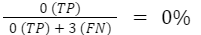

Recall measures the model's ability to find all relevant instances of the positive class (in this case, fraudulent transactions). A recall of 0% means the model fails to identify any of the actual fraudulent transactions. In other words, it misses all of them, labeling them incorrectly as legitimate.
Pros and Cons of Recall:
Pros:
- Focus on Finding All Positives: Recall is crucial when missing positive instances is costly. In medical diagnosis, a false negative could mean a missed opportunity for early treatment.
- Relevance in Anomaly Detection: Recall is valuable in anomaly detection, where identifying rare events is essential.
Cons:
- Neglects True Negatives: Recall doesn't consider true negatives, which can be a drawback in some applications.
- Potential for High False Positives: A model with high recall might also have a high rate of false positives, which can be undesirable in certain scenarios.
Recall and precision often have an inverse relationship. Increasing one might lead to a decrease in the other. Therefore, it's important to choose the metric that aligns with the specific goals and priorities of your classification task.
Here is how each model compares side-by-side:
| Metric | Best Use Cases | Limitations |
|---|---|---|
| Accuracy | Balanced datasets, initial model assessment, general sense of model performance | Not informative in imbalanced classes, treats all errors equally, can be misleading in certain applications |
| Precision | When false positives are costly (e.g., medical diagnosis, spam filtering), information retrieval | Neglects true negatives, can be misleading in imbalanced datasets |
| Recall | When false negatives are costly (e.g., fraud detection, disease screening), anomaly detection | Neglects true negatives, high recall might be accompanied by high false positives, not ideal when false positives are problematic |
Now, let us use all 3 in a simple Logistic Regression model to train on this dataset. We'll use the scikit-learn library to build and train the model.
Model evaluation using accuracy, precision, and recall
We created a balanced dataset that has 50 fraudulent transactions (indicated by 1 in the Is Fraudulent column) and 50 non-fraudulent transactions (indicated by 0). This balance helps the model learn to detect fraud effectively. The transactions cover various merchant types, times of day, days of the week, and locations, providing a diverse set of data for training.
You can see the dataset and the entire code on our GitHub here.
These are the steps we took to in the code:
- Load the Dataset: The dataset is loaded from the CSV file created.
- Prepare the Data: The target variable Is Fraudulent is separated from the features. The categorical variables are converted to dummy variables.
- Split the Data: The data is split into training and testing sets (80% training, 20% testing).
- Create the Model: A Logistic Regression model is created.
- Train the Model: The model is trained on the training data.
- Make Predictions: Predictions are made on the testing data.
- Evaluate the Model: The model is evaluated using accuracy, precision, recall, confusion matrix, and classification report.
These are the results of the training:

The results from the logistic regression model include several key metrics that help evaluate its performance:
Accuracy
- Accuracy: 0.45
- This means that 45% of the total predictions made by the model were correct.
Precision
- Precision: 0.333
- Precision for the class labeled 1 (fraudulent) is 33.3%. This means that out of all the transactions the model predicted as fraudulent, 33.3% were actually fraudulent.
Recall
- Recall: 0.222
- Recall for the class labeled 1 (fraudulent) is 22.2%. This means that out of all the actual fraudulent transactions, the model correctly identified 22.2% of them.
Confusion Matrix

Classification Report
- Class 0 (Non-Fraudulent):
- Precision: 0.50
- Recall: 0.64
- F1-Score: 0.56
- Support: 11 (number of actual non-fraudulent instances)
- Class 1 (Fraudulent):
- Precision: 0.33
- Recall: 0.22
- F1-Score: 0.27
- Support: 9 (number of actual fraudulent instances)
- Overall Metrics:
- Accuracy: 0.45
- Macro Average:
- Precision: 0.42
- Recall: 0.43
- F1-Score: 0.41
- Weighted Average:
- Precision: 0.42
- Recall: 0.45
- F1-Score: 0.43
Analysis
- The model's overall accuracy is low at 45%.
- The precision and recall for the fraudulent class (1) are also low, indicating the model struggles to correctly identify fraudulent transactions.
- The confusion matrix shows that the model is better at predicting non-fraudulent transactions (7 true negatives vs. 4 false positives) than fraudulent ones (2 true positives vs. 7 false negatives).
- The F1-Score, which is the harmonic mean of precision and recall, is low for the fraudulent class (0.27), indicating poor performance in identifying fraud.
The major drawback of this model so far is the size of the dataset. Given how small the sample size is, the model cannot be trained fully to detect fraud.
Note: This should give you a good starting point for training a fraud detection model on your dataset. If you want to improve the model's performance, you can try other algorithms, hyperparameter tuning, feature engineering, etc.
Each metric has its unique way of assessing the model's performance, and by understanding these metrics, you can better interpret the results of our models and make informed decisions about their deployment.
You can train your deep learning models on CUDO Compute. We offer the latest NVIDIA GPUs to speed up your training and inference at the lowest rates. Sign up for free today.
Learn more: LinkedIn , Twitter , YouTube , Get in touch .

Starting from $2.15/hr
NVIDIA H100's are now available on-demand
A cost-effective option for AI, VFX and HPC workloads. Prices starting from $2.15/hr
Subscribe to our Newsletter
Subscribe to the CUDO Compute Newsletter to get the latest product news, updates and insights.