What are Convolutional Neural Networks (CNNs)?

What are Convolutional Neural Networks (CNNs)?

Convolutional Neural Networks (CNNs) are specialized types of neural networks that can automatically and adaptively learn spatial hierarchies of features from inputs, making them exceptionally powerful for tasks involving visual data.

The concept of CNNs isn't new; it dates back to the 1980s with the pioneering work of Yann LeCun and others who introduced the LeNet architecture, primarily for character recognition tasks like reading zip codes and digits.

However, with the introduction of more powerful computing resources like GPUs and the availability of large datasets, CNNs gained widespread adoption and began to demonstrate their full potential. Today, CNNs are a fundamental part of modern deep learning, underlying many of the algorithms that power technologies we use daily.

Source: Saturn Cloud

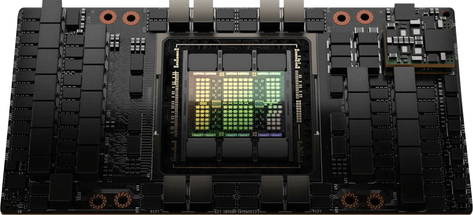
To build and deploy your CNNs faster, use CUDO Compute’s cloud GPUs. CUDO Compute offers the latest NVIDIA GPUs at competitive rates on demand and reserve basis. You can access the NVIDIA H100 starting from $2.79/hour. Get started today!

While the CNNs' ability to handle the complexities of image data and extract meaningful patterns has made them indispensable for researchers and developers alike, they are not only used for visual tasks. Their architecture makes them adaptable to other fields where data exhibits spatial or sequential relationships.

In this article, we will explore spatial hierarchies, why they are important to CNNs, how CNNs process images and their architectures, and how to train them.

What are spatial hierarchies of features in CNNs?

In Convolutional Neural Networks, spatial hierarchies of features describe how the network gradually learns and extracts more complex details from the input data, which is essential to how CNNs perform so well in various tasks.

The process starts with the first layers of the CNN, which identify simple features like edges, corners, and textures. As the data moves through deeper layers, the network combines these basic features to recognize more complex patterns, such as shapes and parts of objects. In the final layers, the CNN can identify whole objects and complete scenes.

Source: Science Direct

Though this hierarchical feature learning is especially effective for images because of their spatial nature, it also works in other fields. For example, in natural language processing (NLP), CNNs can understand the relationships between words and phrases in a sentence. In audio processing, they can learn patterns over time from sound signals.

The core components of convolutional neural networks

A Convolutional Neural Network comprises several key components that work together to process and analyze data, particularly visual data. The primary components include convolutional layers, pooling layers, activation functions, fully connected layers, and sometimes normalization layers. Each of these components has a specific role in processing the input data. Understanding these components is crucial to grasp how CNNs function:

• Convolutional layers: These layers automatically detect features in the input data by applying filters (kernels) across the input image. The filters help capture spatial hierarchies of features like edges, textures, and more complex structures as data moves deeper into the network.
• Pooling layers: After the convolutional layer, pooling layers are typically applied to reduce the spatial dimensions of the feature maps. This process, known as subsampling or down-sampling, helps to decrease the computational load and reduce the risk of overfitting. The most common type of pooling is max pooling, which selects the maximum value from each patch of the feature map, preserving the most important information.

Source: Paper

• Fully connected layers: Following the convolutional and pooling layers, the high-level reasoning in the network is performed by fully connected layers. These layers are similar to those in feedforward neural networks, where each neuron is connected to every neuron in the previous layer. Fully connected layers combine the features extracted by previous layers to make final predictions.
• Activation functions: Activation functions introduce non-linearity into the network, enabling it to learn complex patterns. In CNNs, the most commonly used activation function is the Rectified Linear Unit (ReLU), which replaces negative values with zero while keeping positive values unchanged. ReLU helps to accelerate the convergence of the network during training.

These components are stacked in a CNN to form a deep network that can learn hierarchical representations of the input data. The early layers in a CNN typically learn low-level features like edges, while the deeper layers learn more abstract concepts like shapes and objects.

How CNNs process images

One of the most important things about Convolutional Neural Networks (CNNs) lies in their ability to process and understand images by automatically learning the hierarchical structure of features. Using the model we built in our Feedforward Neural Network article, which we have rebuilt as a CNN. Focusing on the changes made, let’s break down how CNNs process images step by step:

Input layer: The process begins with an input layer where the raw image data is fed into the network. The nature of the input data depends on the type of image. For grayscale images, the input is typically a 2D matrix, where each element in the matrix represents the pixel intensity value of the image. Since the image is in grayscale, there is only one channel (intensity) to consider.

Source: Svitla

For color images, the input is usually a 3D matrix. The first two dimensions represent the spatial dimensions (height and width) of the image, while the third dimension corresponds to the color channels (e.g., Red, Green, and Blue for RGB images). Each pixel in a color image is represented by a combination of three values, one for each channel.

In our code, the input shape is defined when the first layer of the model is added:

model.add(Conv2D(32, (3, 3), activation='relu', input_shape=(128, 128, 3)))`

Here, input_shape=(128, 128, 3) specifies that the input images are 128x128 pixels with 3 color channels (RGB).

Convolution operation: The first convolutional layer in a Convolutional Neural Network (CNN) is responsible for detecting basic features in the input image by applying filters. Each filter in the convolutional layer is essentially a small matrix of weights. During the convolution operation, this filter slides (or "convolves") across the input image, applying a dot product between the filter's weights and corresponding pixel values in the small region of the image.

The result of each convolution is a single number that represents the presence and strength of a specific feature within that region of the image. As the filter moves across the entire image, it generates a 2D output called a "feature map." This map highlights where and how strongly a particular feature (such as an edge, corner, or texture) is detected in different parts of the image.

This is demonstrated in our code by the convolutional layers:

model.add(Conv2D(64, (3, 3), activation='relu'))
model.add(Conv2D(128, (3, 3), activation='relu'))

Each Conv2D layer applies a convolution operation, with the filters learning different aspects of the input image. Multiple filters can be applied in the first convolutional layer, each detecting different types of features. The resulting collection of feature maps captures a diverse set of visual characteristics from the input image.

ReLU activation: After the convolution operation, the ReLU activation function is applied to the resulting feature maps to introduce non-linearity into the model, which is crucial for enabling the network to learn and model complex patterns in the data.

The ReLU function sets all negative values in the feature map to zero while keeping positive values unchanged, which is the non-linearity because the relationship between input and output is no longer a simple linear transformation.

In our code, ReLU activation is applied within the convolutional layers:

model.add(Conv2D(128, (3, 3), activation='relu'))

Without non-linearity, the network would be equivalent to a single linear transformation, no matter how many layers it has. By applying the ReLU function after each convolution, the network can learn more complex patterns and representations in the data, enabling it to capture intricate relationships within the input better.

Pooling: The feature maps are then passed through a pooling layer. The primary purpose of the pooling layer is to reduce the spatial dimensions (height and width) of the feature maps. This is usually done through techniques like max pooling, where the maximum value from a defined region (such as a 2x2 or 3x3 area) is selected and used to represent that region in the pooled feature map.

Source: Saturn Cloud

By selecting the maximum (or, in some cases, average) values, pooling retains the most prominent features within the feature maps while discarding less important information. This reduction in data size also helps decrease the network's computational complexity, making it more efficient.

This is done in our code with max-pooling layers:

model.add(MaxPooling2D(pool_size=(2, 2)))
model.add(MaxPooling2D(pool_size=(2, 2)))
model.add(MaxPooling2D(pool_size=(2, 2)))

Pooling contributes to translational invariance, meaning the network becomes more robust to slight changes in the position of features within the input image. For example, a feature (such as an edge or corner) detected in one part of an image will still be recognized even if it appears in a slightly different location in another image.

Stacking layers: Multiple convolutional and pooling layers are stacked to create deep networks capable of extracting increasingly complex features from the input image. Each successive layer extracts higher-level features from the input image. For example, while the first layer might detect edges, subsequent layers might detect more complex patterns like corners or even objects.

Our code stacks several convolutional and pooling layers to build the network:

model.add(Conv2D(32, (3, 3), activation='relu', input_shape=(128, 128, 3)))
model.add(MaxPooling2D(pool_size=(2, 2)))
model.add(Conv2D(64, (3, 3), activation='relu'))
model.add(MaxPooling2D(pool_size=(2, 2)))
model.add(Conv2D(128, (3, 3), activation='relu'))
model.add(MaxPooling2D(pool_size=(2, 2)))

This stacking allows the model to learn progressively more abstract features.

Flattening and fully connected layers: After several convolutional and pooling layers, the output is flattened into a one-dimensional vector and passed through fully connected layers. These layers combine the features learned by the previous layers to make a final prediction.

In our code, this is handled by the Flatten layer followed by Dense layers:

model.add(Flatten())
model.add(Dense(512, activation='relu'))
model.add(Dropout(0.5))

The Flatten layer converts the 2D matrices into a 1D vector, and the Dense layers act as the fully connected layers, combining the features to make the final decision.

Output layer: Finally, the fully connected layers lead to the output layer, where the network produces a probability distribution over different classes (in the case of classification tasks) or a specific output depending on the task. Your output layer is defined as:

model.add(Dense(2, activation='softmax'))

This Dense layer with softmax activation provides the final classification, outputting the probabilities for each class (e.g., cat or dog).

Through this process, CNNs can analyze images and extract meaningful patterns that can be used for various tasks, from recognizing objects in a photo to diagnosing diseases from medical scans.

Here is the entire code:

import numpy as np
import os
import matplotlib.pyplot as plt
from sklearn.model_selection import train_test_split
from tensorflow.keras.models import Sequential
from tensorflow.keras.layers import Conv2D, MaxPooling2D, Flatten, Dense, Dropout
from tensorflow.keras.optimizers import SGD
from tensorflow.keras.preprocessing.image import ImageDataGenerator
from skimage.transform import resize

# Define dataset path
dataset_path = 'cats-and-dogs'
subdirs = ['train', 'val']  # Subdirectories in the main dataset folder
categories = ['cat', 'dog']  # Categories of images

data = []
img_size = (128, 128)

# Load and preprocess the data
for subdir in subdirs:
    for category in categories:
        path = os.path.join(dataset_path, subdir, category)
        class_num = categories.index(category)
        for img in os.listdir(path):
            try:
                img_path = os.path.join(path, img)
                img_array = plt.imread(img_path)
                img_resized = resize(img_array, img_size, anti_aliasing=True)
                data.append([img_resized, class_num])
            except Exception as e:
                print(f"Failed to load image {img} in {path}: {e}")

# Split data into features (X) and labels (y)
X, y = zip(*data)
X = np.array(X)
y = np.array(y)

# Split the data into training and validation sets
X_train, X_val, y_train, y_val = train_test_split(X, y, test_size=0.2, random_state=42)

print(f"Loaded {len(data)} images")
print(f"Training set: {len(X_train)} images")
print(f"Validation set: {len(X_val)} images")

# Data augmentation
datagen = ImageDataGenerator(
    rotation_range=20,
    width_shift_range=0.2,
    height_shift_range=0.2,
    shear_range=0.2,
    zoom_range=0.2,
    horizontal_flip=True,
    fill_mode='nearest'
)

datagen.fit(X_train)

# Build the CNN model
model = Sequential()

# Convolutional layers
model.add(Conv2D(32, (3, 3), activation='relu', input_shape=(128, 128, 3)))
model.add(MaxPooling2D(pool_size=(2, 2)))

model.add(Conv2D(64, (3, 3), activation='relu'))
model.add(MaxPooling2D(pool_size=(2, 2)))

model.add(Conv2D(128, (3, 3), activation='relu'))
model.add(MaxPooling2D(pool_size=(2, 2)))

model.add(Flatten())  # Flatten the output of the convolutional layers

# Fully connected layers
model.add(Dense(512, activation='relu'))
model.add(Dropout(0.5))  # Add dropout for regularization
model.add(Dense(256, activation='relu'))

# Output layer for classification
model.add(Dense(2, activation='softmax'))

# Compile the model
model.compile(optimizer=SGD(), loss='sparse_categorical_crossentropy', metrics=['accuracy'])

# Train the model
history = model.fit(datagen.flow(X_train, y_train, batch_size=32),
                    validation_data=(X_val, y_val),
                    epochs=10,
                    steps_per_epoch=len(X_train) // 32)

# Evaluate the model
loss, accuracy = model.evaluate(X_val, y_val)
print(f"Validation Accuracy: {accuracy * 100:.2f}%")

# Save the model
model.save('cats_dogs_cnn.keras')

# Load the model to ensure it works
from tensorflow.keras.models import load_model
model = load_model('cats_dogs_cnn.keras')

Common architectures of CNNs

Over the years, several CNN architectures have been developed, each with its unique design and purpose. Let’s explore some of the most influential CNN architectures:

• LeNet-5: Developed by Yann LeCun in the 1990s, LeNet-5 is one of the earliest CNN architectures. It was designed for digit recognition tasks, such as reading handwritten digits in zip codes. LeNet-5 consists of two convolutional layers, followed by two subsampling layers, and finally, two fully connected layers. Despite its simplicity, LeNet-5 laid the groundwork for future CNN architectures.
• AlexNet: Introduced by Alex Krizhevsky and his colleagues in 2012, AlexNet is often credited with popularizing deep learning. It was the first CNN to win the ImageNet Large Scale Visual Recognition Challenge (ILSVRC), achieving a significant improvement in accuracy over previous methods. AlexNet introduced ReLU activation functions and dropout layers to prevent overfitting. It consists of five convolutional layers, followed by three fully connected layers.
• VGGNet: VGGNet, developed by the Visual Geometry Group at the University of Oxford, is known for its simplicity and uniform architecture. It uses small 3x3 filters in each convolutional layer and increases the depth of the network to improve performance. VGGNet achieved state-of-the-art results in the ILSVRC competition and has been widely used in various computer vision tasks.
• ResNet: Residual Networks (ResNet), introduced by Kaiming He and his team at Microsoft in 2015, addressed the problem of vanishing gradients in very deep networks. ResNet introduced residual connections, allowing gradients to flow more easily through the network during training. This innovation enabled the training of extremely deep networks with hundreds or even thousands of layers. ResNet won the ILSVRC 2015 competition and is one of the most influential CNN architectures.
• Inception (GoogleNet): Google introduced the Inception architecture, also known as GoogleNet, in 2014. It introduced the concept of "inception modules," which allow the network to perform convolutions with different filter sizes simultaneously and then concatenate the results. This approach enables the network to capture features at multiple scales and improve performance without significantly increasing computational cost.

These architectures have played a crucial role in advancing the field of computer vision and have influenced the design of many other CNN-based models.

Understanding CNNs is crucial for anyone interested in AI and machine learning, as they form the foundation of many modern applications. Stay updated with our docs and resources, try different convolutional network architectures, and contact us to get access to the latest NVIDIA GPUs on demand and on reserve at CUDO Compute.