Few-shot learning: everything you need to know

Supervised machine learning relies on labeled data to train models, where each input has a designated output. However, manual labeling is expensive, time-consuming, and prone to error, though automated methods still need human supervision.

High-quality labeled data is crucial for model performance, making data acquisition and preparation a bottleneck. In specialized fields like medical diagnostics, expert knowledge is needed for accurate labeling, further increasing the cost and time involved.

Source: Paperwithcode

This challenge has increased the need for few-shot learning, where models learn from limited labeled examples. This approach is particularly relevant in fields where labeled data is scarce or expensive to obtain, such as medical imaging or rare language translation. Few-shot learning aims to mimic human learning, where we can generalize from just a few examples.

In this tutorial, we will discuss few-shot learning, what it is, why it is important, how it works, and its application. Let us begin by discussing what it is.

What is few-shot learning?

Few-shot learning (FSL) is a subfield of machine learning that aims to train models to recognize new classes of data using only a few labeled examples, typically one to five samples per class, starkly contrasting traditional machine learning approaches that often require thousands or even millions of labeled examples to achieve satisfactory performance.

Think of it this way: just as you can recognize other pineapples after seeing one picture, few-shot learning aims to enable models to do the same with minimal examples. The goal of few-shot learning is to enable models to generalize well to new, unseen classes with minimal supervision, which is helpful in scenarios where labeled data is scarce, expensive to obtain, or requires specialized expertise to label.

Source: Paper

For instance, a small online business selling handcrafted jewelry may not have the resources to hire experts to label thousands of images of earrings, necklaces, and bracelets. However, using few-shot learning, they can train a model to categorize their products automatically. By showing the model just a few examples of each type of jewelry, it can learn to recognize and categorize new items with high accuracy.

Few-shot learning algorithms try to mimic how humans learn, where we can quickly generalize from a few examples based on prior knowledge and experience. To better understand how few-shot learning works, it's helpful to familiarize yourself with some key terminologies:

Key terminologies in few-Shot Learning

• Support set: The support set acts as the foundation for few-shot learning. It's a small collection of labeled examples, each representing a different class the model needs to learn. Think of it as a mini-training set, providing the model with just enough information to grasp the key features of each class. During training, the model analyzes these examples to identify patterns, characteristics, and distinctions that will help it classify new, unseen data later on.
• Query set: Once the model has learned from the support set, it's time to test its newfound knowledge. The query set is a collection of unlabeled examples, and the model's task is to predict the correct class for each example based on what it learned from the support set. This simulates a real-world scenario where the model encounters new data it hasn't seen before and must make accurate predictions based on its limited training experience.

Source: Paper

• N-way K-shot Learning: This term describes a standard way of evaluating few-shot learning models. "N" represents the number of different classes the model needs to distinguish between, and "K" represents the number of labeled examples provided for each class in the support set. For instance, a "5-way 1-shot" learning task means the model needs to classify images into five different categories, with only one example of each category available for reference. This setup allows researchers to benchmark and compare different few-shot learning algorithms under controlled conditions.

By using few-shot learning, we can develop more efficient and adaptable machine-learning models that can learn from limited data. Here is why that is important.

Why is few-shot learning important?

Few-shot learning addresses several key challenges in machine learning development, making it a valuable tool for a wide range of applications. Here are some of its most significant benefits:

1. Overcoming data scarcity: In many real-world scenarios, obtaining large amounts of labeled data is simply not feasible. Few-shot learning enables us to train models effectively even when labeled data is limited or expensive to acquire. This opens up new possibilities in domains where data collection is challenging, such as rare diseases, endangered species identification, or specialized equipment maintenance.

2. Reducing labeling costs and time: Traditional machine learning often requires extensive manual labeling efforts, which can be costly and time-consuming. Few-shot learning significantly reduces the need for labeled data, thereby cutting down on labeling costs and accelerating model development timelines.

3. Adapting to new tasks quickly: Few-shot learning models are designed to learn new concepts quickly with minimal supervision. This adaptability allows them to be easily fine-tuned for new tasks or domains without requiring extensive retraining. This is particularly valuable in dynamic environments where new data or tasks emerge frequently.

4. Democratizing machine learning: By reducing the reliance on large labeled datasets, few-shot learning makes machine learning more accessible to smaller organizations and individuals who may not have the resources to collect and label massive datasets.

Source: Paper

5. Addressing long-tail problems: In many real-world datasets, a few classes dominate the majority of examples, while many other classes have very few instances. This is known as the long-tail problem. Few-shot learning is well-suited to address this issue, as it can effectively learn to recognize rare classes with limited examples.

6. Improving generalization: Few-shot learning encourages models to focus on learning generalizable features rather than memorizing specific examples, often leading to better performance on unseen data and improved robustness to variations in data distribution.

In summary, few-shot learning has the potential to revolutionize the way we approach machine learning, making it more efficient, adaptable, and accessible. Its ability to learn from limited data opens up exciting new possibilities in various fields.

In the next section, we will delve into the inner workings of few-shot learning and explore the different approaches used to achieve it.

How does few-shot learning work?

There are several methods for implementing few-shot learning in a project, each with unique strategies to tackle the challenge of learning from a limited number of labeled examples. Here are some of the most prominent methods:

1. Meta-learning: Meta-learning, or "learning to learn," involves training a model on a variety of tasks so it can quickly adapt to new tasks with few examples. This approach helps the model develop prior knowledge that can be fine-tuned for specific tasks during the testing phase. Techniques like Model-Agnostic Meta-Learning (MAML) fall under this category.
2. Metric learning: Metric learning focuses on learning a distance metric so that the model can classify new examples based on their similarity to known examples. Methods like Prototypical Networks and Matching Networks are popular in this domain. These models learn an embedding space where similar examples are clustered together, making classification straightforward based on distance measures.
3. Data augmentation: This method involves artificially increasing the number of training examples through techniques like flipping, cropping, adding noise, or using generative models like GANs (Generative Adversarial Networks) to create synthetic data. This helps mitigate the issue of having too few examples by providing more varied training data.
4. Transfer learning: Transfer learning leverages pre-trained models on large datasets and fine-tunes them on the few-shot tasks. This allows the model to use learned features from the large dataset, reducing the need for extensive data in the new task. Fine-tuning or using the pre-trained model as a feature extractor are common approaches in transfer learning.
5. Memory-augmented networks: These networks, like Neural Turing Machines, incorporate an external memory that allows the model to store and recall information from a few examples. During testing, the model uses this memory to make predictions based on the small amount of available data.
6. Adversarial feature hallucination: This technique involves generating additional training examples by creating variations of the few available examples. Adversarial networks are used to produce these variations, helping the model generalize better from limited data.

These methods can be combined or adapted depending on the specific requirements of the project and the nature of the data. The choice of method often depends on the balance between computational resources, the complexity of the task, and the available data. In this article, we will focus on how to use the metric learning method.

Implementation methods for metric learning

Metric learning is a fundamental approach in few-shot learning that aims to learn a representation space where similar instances are close to each other and dissimilar instances are far apart. This technique is in few-shot learning scenarios where there are limited labeled examples for each class. There are few ways ways to implement this. Let’s break them down.

The main implementation methods for metric learning in few-shot learning can be broadly categorized into several approaches, which include learning feature embeddings, learning distance or similarity measures, and sometimes hybrid methods that combine elements of both. Here are the primary methods in detail:

1. Learning feature embeddings:
   • Task-agnostic embedding models: These models aim to learn a generalizable feature representation that works well across various tasks. The idea is to create a robust feature extractor that can differentiate between classes based on learned features, regardless of the specific task at hand.
   • Task-specific embedding models: These models are fine-tuned for specific tasks, enhancing the ability to distinguish between the classes involved in the particular few-shot learning scenario. They often use techniques like data augmentation and multi-task learning to improve performance despite limited data.
2. Learning distance or similarity measures:

Source: Paper

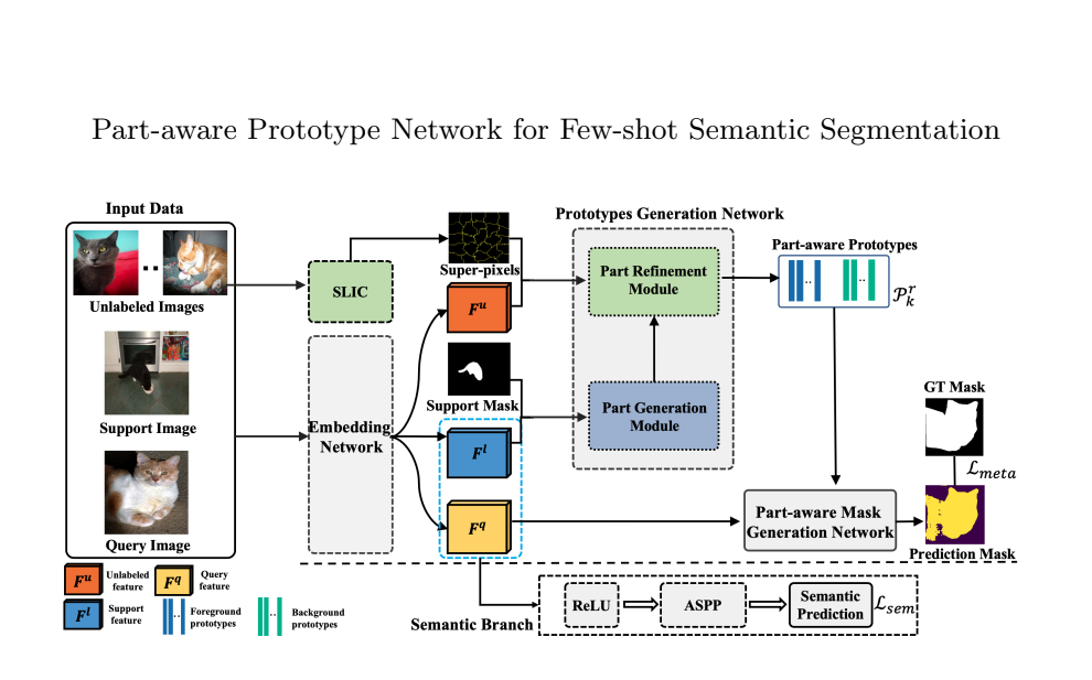
• Prototypical networks: This method involves computing a prototype (or centroid) for each class in the embedding space. Classification of new instances is then done by measuring the distance between these class prototypes. It’s effective and computationally simple.
• Relation networks: These networks learn a deep non-linear function to measure similarity between instances. Instead of using a predefined distance metric, the network learns to compare query instances with support instances, thus capturing complex relationships.
• Matching networks: These networks use a weighted nearest neighbor classifier to compare a query instance to the labeled instances in the support set. The key idea is to learn an embedding where instances from the same class are closer to each other than to instances from different classes.

3. Hybrid methods:
   • Two-stage approaches: These combine metric learning with meta-learning components. For instance, the first stage might focus on learning a robust feature representation, while the second stage involves fine-tuning the distance metrics or classifiers using meta-learning techniques to adapt quickly to new tasks.

These methods provide a solid foundation for implementing metric learning in few-shot learning scenarios, enabling models to perform well even with limited labeled data.

Let us see an example of how the matching networks are implemented.

Matching networks

Implementing Matching Networks for few-shot learning involves several key steps, each with its own purpose and functionality. We trained the model to recognize cats and dogs. Below is a detailed explanation of each step we took to train the model using this dataset from Kaggle, which holds images of cats and dogs.

Step 1: Data preparation

First, we organized images into a structure that facilitates easy loading and labeling. The images are stored in directories, each representing a different class (e.g., one folder for cat images and another for dog images).

This directory structure helps in creating datasets that are easy to manipulate and use for training models.

class CatsDogsDataset(Dataset):
    def __init__(self, root_dir, transform=None):
        self.root_dir = root_dir
        self.transform = transform
        self.classes = [d for d in os.listdir(root_dir) if os.path.isdir(os.path.join(root_dir, d))]
        self.filepaths = []
        self.labels = []

        for class_idx, class_name in enumerate(self.classes):
            class_dir = os.path.join(root_dir, class_name)
            for img_name in os.listdir(class_dir):
                img_path = os.path.join(class_dir, img_name)
                if img_name.lower().endswith(('png', 'jpg', 'jpeg')):
                    self.filepaths.append(img_path)
                    self.labels.append(class_idx)

    def __len__(self):
        return len(self.filepaths)

    def __getitem__(self, idx):
        img_path = self.filepaths[idx]
        image = Image.open(img_path).convert('RGB')
        label = self.labels[idx]
        if self.transform:
            image = self.transform(image)
        return image, label

The init method initializes the dataset object, loading the image paths and their corresponding labels, the len method returns the total number of images in the dataset, and the getitem method loads and returns an image and its label by index, applying any specified transformations.

Next, we ensure that the images are consistent and that the model's robustness is enhanced through augmentation. Images are resized, augmented (e.g., flipped, rotated), and normalized to standardize the input data.

transform = transforms.Compose([
    transforms.Resize((224, 224)),
    transforms.RandomHorizontalFlip(),
    transforms.RandomRotation(15),
    transforms.ColorJitter(brightness=0.2, contrast=0.2, saturation=0.2, hue=0.1),
    transforms.RandomResizedCrop(224, scale=(0.8, 1.0)),
    transforms.ToTensor(),
    transforms.Normalize((0.485, 0.456, 0.406), (0.229, 0.224, 0.225))
])

Using Resizing ensures all images are the same size (224x224 pixels), then Random Horizontal Flip and Rotation introduces variability in the training data, helping the model generalize better. We then apply Color Jitter to adjust brightness, contrast, saturation, and hue to simulate different lighting conditions. Finally, Normalization standardizes the pixel values based on mean and standard deviation values typically used for pre-trained models like ResNet.

Step 2: Custom dataset classes

In our next step, we create support and query sets required for few-shot learning tasks. The dataset is divided into support and query sets. The support set contains a few examples from each class (k-shot), and the query set contains the remaining examples.

class FewShotDataset(Dataset):
    def __init__(self, dataset, n_way, k_shot, mode='train'):
        self.dataset = dataset
        self.n_way = n_way
        self.k_shot = k_shot
        self.mode = mode
        self.class_indices = {cls: [] for cls in range(n_way)}

        for idx, (_, label) in enumerate(dataset):
            if label < n_way:
                self.class_indices[label].append(idx)

        self.support_set = []
        self.query_set = []
        self._create_few_shot_task()

    def _create_few_shot_task(self):
        for cls in range(self.n_way):
            indices = random.sample(self.class_indices[cls], self.k_shot * 2)
            self.support_set.extend(indices[:self.k_shot])
            self.query_set.extend(indices[self.k_shot:])

    def __len__(self):
        return len(self.support_set) if self.mode == 'train' else len(self.query_set)

    def __getitem__(self, idx):
        if self.mode == 'train':
            img_idx = self.support_set[idx]
        else:
            img_idx = self.query_set[idx]
        img, label = self.dataset[img_idx]
        return img, label

Using the init method to initialize the dataset, dividing it into support and query sets based on the specified number of classes (n_way) and examples per class (k_shot), we then randomly select indices for support and query sets, and define the length and item retrieval for the dataset.

Step 3: Model definition

The third step extracts feature embeddings from images using a pre-trained model. ResNet-18, a popular convolutional neural network pre-trained on ImageNet used for feature extraction, is used as the base encoder, modified to produce lower-dimensional embeddings.

class EnhancedResNetEncoder(nn.Module):
    def __init__(self):
        super(EnhancedResNetEncoder, self).__init__()
        self.resnet = models.resnet18(pretrained=True)
        self.resnet.fc = nn.Identity()  # Remove the final fully connected layer
        self.fc = nn.Linear(512, 128)   # Add a new fully connected layer

    def forward(self, x):
        x = self.resnet(x)
        x = self.fc(x)
        return x

Removing the final layer, we replace it with a a custom layer to reduce the feature dimensionality to 128, then use the forward method to define how the input data passes through the network layers to produce embeddings.

Using a matching network, we cassify query images based on their similarity to support images. The network uses the encoder to embed support and query images and then computes similarities between these embeddings to classify the query images.

class MatchingNetwork(nn.Module):
    def __init__(self, encoder):
        super(MatchingNetwork, self).__init__()
        self.encoder = encoder

    def forward(self, support, query, n_way, k_shot):
        support_embeddings = self.encoder(support)
        query_embeddings = self.encoder(query)
        support_embeddings = support_embeddings.view(n_way, k_shot, -1).mean(1)
        similarities = torch.matmul(query_embeddings, support_embeddings.t())
        return similarities

The encoder generates embeddings for both support and query images. For each class, the embeddings of the support images are averaged to create a class prototype. Similarities between query embeddings and class prototypes are computed using a dot product, resulting in similarity scores used for classification.

Step 4: Training and evaluation

In this step, we load the support and query sets in batches for training. Data loaders are created for the support and query sets using a PyTorch utility that creates an iterable over the dataset, allowing batch processing and shuffling of data for training, which enables efficient batch processing during training and evaluation.

train_dataset_path = 'cats-and-dogs/train'
val_dataset_path = 'cats-and-dogs/val'
train_dataset = CatsDogsDataset(root_dir=train_dataset_path, transform=transform)
val_dataset = CatsDogsDataset(root_dir=val_dataset_path, transform=transform)
n_way = 2  # Number of classes (cats and dogs)
k_shot = 5  # Number of images per class for support set

support_set = FewShotDataset(train_dataset, n_way, k_shot, mode='train')
query_set = FewShotDataset(val_dataset, n_way, k_shot, mode='val')
support_loader = DataLoader(support_set, batch_size=n_way * k_shot, shuffle=True)
query_loader = DataLoader(query_set, batch_size=n_way * k_shot, shuffle=True)

The model is trained over multiple epochs, optimizing the loss function to improve the similarity-based classification of query images.

encoder = EnhancedResNetEncoder()
model = MatchingNetwork(encoder)
optimizer = optim.Adam(model.parameters(), lr=0.0001)  # Adjusted learning rate
criterion = nn.CrossEntropyLoss()

Let's delve into each step with greater detail:

for epoch in range(50):  # Increased number of epochs
    for support, query in zip(support_loader, query_loader):
        support_imgs, support_labels = support
        query_imgs, query_labels = query

        optimizer.zero_grad()
        similarities = model(support_imgs, query_imgs, n_way, k_shot)
        loss = criterion(similarities, query_labels)
        loss.backward()
        optimizer.step()

        print(f'Epoch {epoch}, Loss: {loss.item()}')

We initialize the encoder (EnhancedResNetEncoder) and the matching network (MatchingNetwork) with the encoder. An Adam optimizer is used to update the model parameters, and a cross-entropy loss function is employed to calculate the loss between the predicted and true labels.

The training runs for a specified number of epochs (e.g., 50), iterating through the entire dataset multiple times to optimize the model. The zip function is used to iterate over the support and query data loaders in parallel, fetching batches of support and query images.

For each batch, the model computes the similarity scores between query and support images. The cross-entropy loss is calculated between the similarity scores and the true labels of the query images. The gradients are then computed with loss.backward(), and the optimizer updates the model parameters using optimizer.step().

After training, the model's accuracy is evaluated by comparing predicted labels with true labels of the query set.

with torch.no_grad():
    correct = 0
    total = 0
    for support, query in zip(support_loader, query_loader):
        support_imgs, support_labels = support
        query_imgs, query_labels = query

        similarities = model(support_imgs, query_imgs, n_way, k_shot)
        predicted_labels = torch.argmax(similarities, dim=1)
        correct += (predicted_labels == query_labels).sum().item()
        total += query_labels.size(0)

    accuracy = correct / total
    print(f'Accuracy: {accuracy * 100:.2f}%')

The torch.no_grad() context is used to disable gradient calculations, reducing memory usage and speeding up computations during evaluation. Similar to training, support and query sets are processed in batches. he model computes the similarity scores for query images against the support set.

The predicted labels for query images are obtained by finding the class with the highest similarity score (torch.argmax(similarities, dim=1)) and the number of correct predictions is summed and divided by the total number of query images to compute accuracy.

Summary

Matching Networks uses the principles of metric learning to classify new instances based on their proximity to known instances in an embedding space, making them effective for few-shot learning scenarios.

Application of few-shot learning

Image Recognition

Challenges and solutions: Traditional image recognition models require large datasets to achieve high accuracy. Few-shot learning addresses this by enabling models to recognize new categories with only a few labeled images. Techniques like prototypical networks and Siamese networks are particularly effective in this domain.

Examples from industry: Companies like Google and Facebook use few-shot learning for tasks such as image classification, object detection, and facial recognition. These models can quickly adapt to new categories, making them valuable for dynamic and diverse datasets.

Natural language processing (NLP)

Importance in NLP tasks: Few-shot learning is crucial in NLP tasks where labeled data is scarce. It allows models to understand and process new languages or dialects with minimal training data. Techniques like matching networks and MAML are often used to achieve this.

Case studies: Few-shot learning has been applied to tasks such as machine translation, text classification, and sentiment analysis. For example, OpenAI's GPT-3 model demonstrates few-shot capabilities by performing various NLP tasks with minimal examples.

Healthcare

Impact on medical diagnostics: Few-shot learning has significant potential in healthcare, particularly in diagnosing rare diseases. Traditional models require large datasets, which are often unavailable for rare conditions. Few-shot learning enables models to learn from a few medical records, improving diagnostic accuracy.

Specific examples and research: Research studies have demonstrated the effectiveness of few-shot learning in medical imaging, such as classifying medical images and detecting anomalies. Companies are also developing few-shot learning models for personalized medicine, where individual patient data is limited.

Robotics

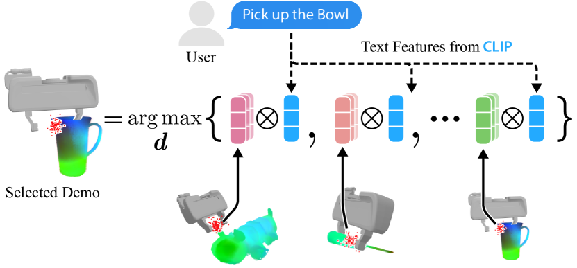
Teaching robots new tasks: Few-shot learning enables robots to learn new tasks with minimal demonstrations. This is particularly valuable in industrial settings where reprogramming robots for new tasks is costly and time-consuming.

Source: Paper

Practical implementations: Researchers have developed few-shot learning models for robotic manipulation, allowing robots to quickly adapt to new objects and tasks. These models use techniques like MAML to efficiently generalize from previous experiences and learn new skills.

Conclusion

Few-shot learning represents a significant advancement in the field of machine learning, enabling models to learn new tasks with minimal data. By using meta-learning, embedding models, and various innovative approaches, few-shot learning has shown great promise in applications ranging from image recognition and NLP to healthcare and robotics.

Sign up to CUDO Compute to use few-shot learning without fear of overfitting or other machine learning issues. We offer the latest NVIDIA GPUs at affordable rates. You can sign up to use the NVIDIA A100 and H100 today or register your interest in the NVIDIA H200 and B100 as soon as they are available.